Question 3 on the G-Research Sample Quant Exam:
A stock has beta of
and stock specific daily volatility of
. Suppose that yesterday’s closing price was
and today the market goes up by
- What’s the probability of today’s closing price being at least
?
- What’s the probability that the closing price is at least
?
Generally, stock returns are modeled using a normal distribution. This is because the Central Limit Theorem says that the sum of many small, independent random variables tends to be normally distributed. As a result, daily stock price movements, influenced by a variety of small, independent factors, thus follow a normal distribution. (Stock prices, on the other hand, follow a log-normal distribution – but this is another topic.)
Let ![]() denote a random variable representing the stock’s returns. Then
denote a random variable representing the stock’s returns. Then
![]()
We already know that ![]() . To calculate
. To calculate ![]() , note that the beta,
, note that the beta, ![]() , represents the stock’s sensitivity to the market (note that
, represents the stock’s sensitivity to the market (note that ![]() can be negative in some cases). Hence, we just use the formula
can be negative in some cases). Hence, we just use the formula
![]()
For a stock’s current price to reach a target price, it needs a return of
![]()
Now we can calculate the probability. It is given by
![]()
![]()
![]()
In the general case, given a stock’s currence price (![]() ), target price (
), target price (![]() ), beta (
), beta (![]() , idiosyncratic volatility (
, idiosyncratic volatility (![]() ), and the market’s expected return (
), and the market’s expected return (![]() ), we can compute the probability that the stock hits the target price (if
), we can compute the probability that the stock hits the target price (if ![]() ) or drops below it (if
) or drops below it (if ![]() ).
).
First define ![]() and
and ![]() . Then
. Then
![]()
![]()
Using our new formulas, the probability that the stock in the original problem statement exceeds the price of ![]() per share is
per share is
![]()
We can actually code this using Python.
import numpy as np
import scipy.stats as stats

# Given data
beta = 2.0  # Stock's sensitivity to the market
market_return = 0.01  # Market's expected return
sigma = 0.02  # Idiosyncratic volatility
p_c = 100  # Current price
mu = beta * market_return  # Stock's expected return

# 103 case:
p_t_103 = 103 # Target prices (p_t)
x_103 = (p_t_103 / p_c) - 1 # Required returns (x)
p_at_least_103 = 1 - stats.norm.cdf(x_103, mu, sigma) # P(R > x) - use a built in CDF function
print(f"Probability that today's closing price is at least 103: {p_at_least_103:.2%}") # Print odds

# 110 case:
p_t_110 = 110 # Target prices (p_t)
x_110 = (p_t_110 / p_c) - 1 # Required returns (x)
p_at_least_110 = 1 - stats.norm.cdf(x_110, mu, sigma) # P(R > x) - use a built in CDF function
print(f"Probability that today's closing price is at least 110: {p_at_least_110:.2%}") # Print odds
This is a good check that our work makes sense. However, it starts to become very interesting when we generalize all of this.
Below is a function that takes a stock and a target price (and optionally the market index) as inputs and calculates the probability that the stock hits the target price.
import yfinance as yf
import numpy as np
import scipy.stats as stats
from datetime import datetime, timedelta
import statsmodels.api as sm

def stock_price_probability_calculator(stock, target_price, market = "^GSPC"):
    '''Takes in a stock symbol (str), a target price (float), and market symbol (str) that is preset to the S&P500'''

    def returns(ticker): # Enter a valid stock symbol
        start_date = datetime.now() - timedelta(days=90) # Can change this to see a different range
        end_date = datetime.now()
        data = yf.download(tickers=ticker, start=start_date, end=end_date, interval='1d')
        returns = data['Adj Close'].pct_change().dropna()
        return returns

    stock_returns = returns(stock)
    market_returns = returns(market)

    def beta(stock_returns, market_returns):
        covariance_matrix = np.cov(stock_returns, market_returns)
        beta = covariance_matrix[0, 1] / covariance_matrix[1, 1]
        return beta

    beta = beta(stock_returns, market_returns)

    # Calculate idiosyncratic volatility by regressing stock returns on market returns
    def idiosyncratic_volatility(stock_returns, market_returns):
        X = sm.add_constant(market_returns)
        model = sm.OLS(stock_returns, X).fit()
        residuals = model.resid
        idiosyncratic_volatility = residuals.std()
        return idiosyncratic_volatility

    idiosyncratic_volatility = idiosyncratic_volatility(stock_returns, market_returns)

    # Last price and day of stock and market
    live_stock_data = yf.download(tickers=stock, period='1d', interval='1m')
    live_market_data = yf.download(tickers=market, period='1d', interval='1m')
    latest_stock_price = live_stock_data['Adj Close'].iloc[-1]
    latest_stock_date = live_stock_data.index[-1]
    latest_market_price = live_market_data['Adj Close'].iloc[-1]
    latest_market_date = live_market_data.index[-1]

    avg_market_return = market_returns.mean()

    mu = beta * avg_market_return
    sigma = idiosyncratic_volatility
    x = (target_price / latest_stock_price) - 1 # Stock return needed to reach target price

    if target_price > latest_stock_price:
        probability = 1 - stats.norm.cdf(x, mu, sigma)
    else:
        probability = stats.norm.cdf(x, mu, sigma)

    print("\n[Data Retrieval Complete]\n")
    print(f"Latest Price of {stock}: {latest_stock_price:.2f} at {latest_stock_date.now()}")
    print(f"Latest Price of {market}: {latest_market_price:.2f} at {latest_market_date.now()}")
    print(f"Beta of {stock}: {beta:.2f}")
    print(f"Idiosyncratic Volatility of {stock}: {idiosyncratic_volatility:.2%}")
    print(f"Average Market Return: {avg_market_return:.2%}")
    if target_price > latest_stock_price:
        print(f"Probability that {stock} will close at least at {target_price}: {probability:.2%}\n")
    else:
        print(f"Probability that {stock} will close under {target_price}: {probability:.2%}\n")

stock_price_probability_calculator("SMCI", 680.00) # Example
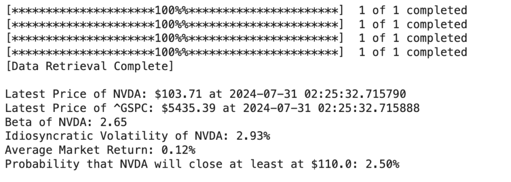
For example, Nvidia (NVDA) close at ![]() per share today (July 30, 2024). What is the probability that it closes at
per share today (July 30, 2024). What is the probability that it closes at ![]() per share tomorrow?
per share tomorrow?
stock_price_probability_calculator("NVDA", 110.00)
Disclaimer: This is not investment advice. 🙂
GitHub repository: https://github.com/trippytrung/Stock-Price-Probability-Calculator

